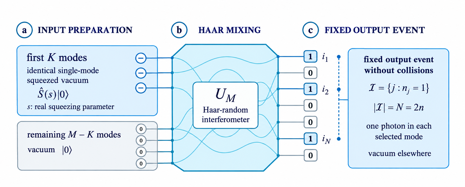
How can counting photons become a difficult computational problem? The answer connects quantum interference to two matrix functions, the permanent and the hafnian. Turning that connection into a robust statement about classical computation requires probability theory as well as complexity theory.
In my recent work, I prove uniform matrix-law hiding for the finite Gaussian transpose-Gram reference and local hafnian anticoncentration with a quadratic small-ball bound. These results address two analytic obstacles in Gaussian boson sampling (GBS). The exact statements and parameter ranges matter: they are ingredients for hardness arguments, and do not by themselves prove a complete quantum advantage theorem. 10, 11
This post starts with ordinary boson sampling, explains the conjectures behind its hardness argument, and then shows where my GBS results enter. References and theorem numbers are collected at the end.
1. Boson sampling begins with interference
Prepare $N$ indistinguishable photons, one in each of $N$ input modes of an $M$-mode interferometer. An optical mode is a distinguishable channel, such as a spatial path. A unitary matrix $U$ describes how the interferometer mixes these channels. At the output, detectors count photons.
For a collision-free input set $T$ and output set $\mathcal I$, both of size $N$, the ideal probability is
The permanent sums over all assignments of inputs to outputs,
For two photons, $\operatorname{Per}(X)=X_{11}X_{22}+X_{12}X_{21}$. We add the complex amplitudes before taking the squared modulus. Their phases can reinforce or cancel each other. This is why independently routing classical particles does not reproduce the same probabilities. 1
The computational task is to generate output patterns with the right probabilities. A device need not print a permanent. Also, an exponentially large sum is not itself a proof that every algorithm must take exponential time. The relevant hardness statements come from computational reductions.
2. Two different questions behind the hardness argument
The Gaussian reference for ordinary boson sampling is $X\in\mathbb C^{N\times N}$ with independent standard circular complex Gaussian entries. Here $\mathbb E|X_{ij}|^2=1$, and
Two questions should be kept separate.
Average-case hardness asks whether typical instances are difficult. Aaronson and Arkhipov's Permanent-of-Gaussians Conjecture concerns approximating the complex permanent on most Gaussian inputs to relative error. Worst-case exact hardness alone does not establish that claim. 1, Conjecture 1.5
Anticoncentration asks whether the answer is usually large enough for relative accuracy to be meaningful. Their Permanent Anti-Concentration Conjecture asks for a polynomial $q$ such that
An additive error of $10^{-8}$ is useful for a probability of $10^{-5}$, but potentially useless for a probability of $10^{-20}$. Anticoncentration controls this small-denominator problem. It does not require every outcome to have roughly the same probability.
A 2026 development. Koehler and Leung's preprint reports a proof of the permanent anticoncentration conjecture. In the complex case, its center-uniform bound has the form
for a universal constant $C$. Thus a current account should describe the famous conjecture historically and acknowledge this reported resolution, rather than present it as untouched. The average-case hardness assumption remains separate. Their Fourier compression method also informs my hafnian proof. 2, 11
The ordinary boson sampling roadmap
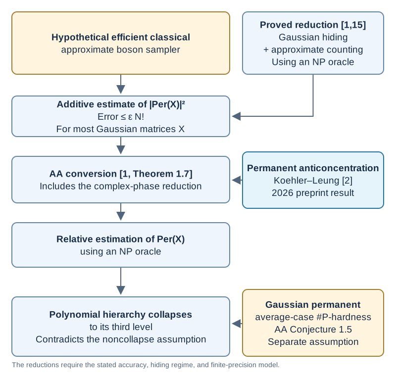
Stockmeyer's approximate counting theorem uses an NP oracle to estimate a classical sampler's probabilities. Gaussian hiding connects appropriate interferometer coordinates to random matrix instances. The conversion from squared magnitude to the complex permanent additionally uses the reduction in Aaronson and Arkhipov's Theorem 1.7, not simply division by a lower bound. 1, 15
The polynomial hierarchy is a family of complexity classes extending NP. Its noncollapse is the complexity assumption used to rule out the sampler after the other ingredients are supplied. This is a conditional argument, not a theorem that every noisy optical device defeats every classical computer.
3. Gaussian boson sampling replaces single photons by squeezed light
GBS uses Gaussian optical states as inputs, followed by photon counting. The word Gaussian describes the optical state before detection; it does not mean that the resulting photon counts have a Gaussian distribution. Hamilton and colleagues established the hafnian probability formula, and Kruse and colleagues developed the detailed framework. 3, 4
For the model considered here, the first $K$ modes contain identical squeezed vacuum states and the other $M-K$ modes contain vacuum. I write the squeezing parameter as $s>0$, using the convention
Here $a^\dagger$ creates a photon and $a$ annihilates one. Squeezed vacuum contains a superposition of even photon numbers. After a passive interferometer, a lossless output therefore still has even total photon number. In the selected sector, write $N=2n$.
| Symbol | Meaning |
|---|---|
| $M$ | Total optical modes |
| $K$ | Inputs with the common squeezing parameter $s$ |
| $N=2n$ | Photons in the selected collision-free output event |
| $\mathcal I$ | Selected output modes, with one photon in each |
| $V=U_{\mathcal I,[K]}$ | The corresponding $N\times K$ interferometer block |
The physical kernel is the complex symmetric matrix $A=VV^{\mathsf T}$, and the ideal event probability is
This is the probability of the event in the full ideal experiment, not a probability renormalized after conditioning on total photon number $N$. The mean input photon number is $K\sinh^2(s)$, so whether a chosen sector is common also depends on $s$. 4, 11
The hafnian sums over perfect pairings of $2n$ indices,
For four indices it is $A_{12}A_{34}+A_{13}A_{24}+A_{14}A_{23}$. The pairing structure reflects the photon-pair structure of squeezed inputs.
Throughout, $\mathsf T$ means ordinary transpose. The product $VV^{\mathsf T}$ is generally neither Hermitian nor positive semidefinite.
4. Hiding is a random matrix problem of its own
A Gaussian matrix is easier to analyze than a block of a Haar-random unitary. But the kernel in GBS is a product of a block and its transpose. Its entries share Gaussian factors and remain dependent at finite $K$. Approximating the entire block by independent entries can fail in dense input regimes even when an approximation of the product remains useful.
Deshpande and colleagues made this hiding obstacle explicit in GBS hardness arguments. Shou, Miller, and Galitski subsequently proved hiding results including the fully squeezed case. Shou, Gorshkov, Galitski, and Miller then addressed arbitrary numbers of squeezed inputs in the range $N\leq K\leq M$. My contribution strengthens the quantitative guarantee and extends its finite-dimensional domain. 5, 8, 9, 10
My uniform finite-dimensional bound
Let $G\in\mathbb C^{N\times K}$ have independent standard circular complex Gaussian entries. My updated uniform hiding theorem holds for every $1\leq N\leq M$ and $1\leq K\leq M$, including $K<N$,
Here $d_{\mathrm{TV}}(\mu,\nu)=\sup_E|\mu(E)-\nu(E)|$. The statement keeps one finite transpose-Gram target, with a bound independent of the number of squeezed inputs $K$. In particular, $N^2/M\to0$ suffices for the bound to vanish uniformly over $1\leq K\leq M$. The explicit constant is large; this is a rigorous mathematical guarantee, not an optimized experimental size requirement. 10, updated theorem
Uniformity refers to the parameter $K$ and to every fixed selected block. It does not assert a joint approximation of exponentially many output probabilities. Also, this theorem compares matrix laws; by itself it does not give an efficient procedure that embeds a prescribed Gaussian instance into a Haar interferometer.
What improves over earlier hiding bounds?
To my knowledge, this is the first explicit $O(N^2/M)$ total-variation hiding bound for the finite transpose-Gram target that is uniform in $K$ over the full admissible range $1\leq N,K\leq M$. This is the largest possible parameter domain for an $N\times K$ block of an $M\times M$ interferometer. The finite inequality holds throughout that domain; it guarantees a small error when $615172N^2/M$ is small. 10, updated theorem
The following comparison keeps the reference laws explicit. The earlier sparse bound is restated in Shou and colleagues' equation (3.1); their Theorems 1.1–1.2 give the symmetric-Gaussian bounds. 8, 9
| Hiding guarantee | Reference law | Sufficient condition for the displayed error bound to vanish |
|---|---|---|
| Earlier sparse bound: $O(\sqrt{NK/M})$, for $N\leq K$ | Finite transpose-Gram $GG^{\mathsf T}/\sqrt K$ | $NK/M\to0$ |
| Earlier dense bound: $O(N/\sqrt K)$, for $N\leq K$ | Independent symmetric Gaussian | $N^2/K\to0$ |
| My bound: $\min\{1,615172N^2/M\}$, for all $1\leq N,K\leq M$ | Finite transpose-Gram $GG^{\mathsf T}/\sqrt K$ | $N^2/M\to0$, uniformly in $K$ |
In the shared range $N\leq K\leq M$, the comparison follows from
Thus either cited earlier condition implies my convergence condition, while the converse fails. For example, take $K=N^2$ and $M=N^3$ as $N\to\infty$. My error bound is $615172/N\to0$, whereas $NK/M=N^2/K=1$. This example shows a strict enlargement of the regime certified by these displayed bounds. It does not show that the underlying distances in the earlier results fail to converge.
The improvement concerns a uniform convergence guarantee for the finite transpose-Gram target. Passing to an independent symmetric Gaussian target still requires an additional comparison, supplied by 9, Theorem 1.2 when $N^2/K\to0$. An asymptotic comparison also does not establish the smallest numerical error bound at every finite parameter choice.
5. My local anticoncentration theorem
To my knowledge, I give the first unconditional, explicit, center-uniform quadratic small-ball bound for finite complex Gaussian transpose-Gram hafnians in the GBS setting. The theorem below specifies its parameter range. “Unconditional” means that the probability theorem assumes no computational hardness or unproved anticoncentration conjecture. Earlier moment results establish weak anticoncentration, which is a different guarantee. 6, 7, 11, 13
Write $X=G^{\mathsf T}\in\mathbb C^{K\times2n}$ and
The exact second moment was established in the earlier moment analysis by Ehrenberg and colleagues; it supplies the natural scale for the theorem. 6, 7
For $n\geq1$ and $K\geq4n$, my local theorem gives
with the explicit coefficient
The product is one when $n=1$. The coefficient grows at most polynomially when $n^2/K=O(\log n)$. The finite condition $K\geq4n$ alone is not a claim of a polynomial coefficient at the boundary. 11, Theorem 2.1 and Corollary 2.6
What does the bound say? A disk of radius $\varepsilon$ in the complex plane has area proportional to $\varepsilon^2$. My result obtains this quadratic power uniformly over the disk center, with an explicit dimension-dependent multiplier. At $z=0$, it controls exceptionally small amplitudes. It is stronger in this local sense than a statement that the amplitude is moderately large with merely an inverse-polynomial probability.
What makes the proof difficult? Conditioning on a Gaussian column turns the hafnian into a complex Gaussian variable with a random variance. Its cofactors depend on the same Gaussian matrix that generates that variance. The proof combines Fourier compression, drawing on Koehler and Leung, with a conditional Wishart identity that preserves the transpose-Gram coordinate. That preservation is what permits control of the dependent inverse variance. 2, 11
The independent symmetric Gaussian limit
For a $2n\times2n$ complex symmetric Gaussian matrix $Y$, whose entries above the diagonal are independent standard circular complex Gaussians, the corresponding result is
The diagonal does not enter a hafnian without loops. For the matrix ensemble used in the limit, its independent diagonal entries have complex variance two. The bound supplies a polynomial Gaussian lower-tail estimate of the kind needed in the original hafnian proposals. It does not prove an average-case hardness conjecture or recover a complex phase from a squared modulus. 3, 4, 11, Theorem 2.3 and Corollary 2.5
How this relates to weak anticoncentration
Ehrenberg and colleagues developed the moment framework and identified transitions in weak anticoncentration. My exact-moment preprint and independent work by Shou and colleagues locate the $n^2/\log n$ scale for the moment criterion. These results motivate the regime, but a second/fourth-moment ratio does not itself control every arbitrarily small disk. The local theorem supplies that additional control. 6, 7, 12, 13
6. Putting hiding and anticoncentration together
For a fixed output set $\mathcal I$, take $N=2n$ and $4n\leq K\leq M$. Total variation controls the inverse image of any event under the hafnian. Combining the two theorems therefore yields
This is the finite-Haar consequence in my local anticoncentration manuscript. It applies to the ideal model with common squeezing, zero displacement, and a specified collision-free event. 11, Corollary 2.7
Define a Gaussian reference scale for the physical probability,
Because a hafnian of order $2n$ is homogeneous of degree $n$, we obtain
This reference scale is not being asserted to equal the exact Haar mean probability. It is the explicitly normalized Gaussian scale used in the comparison.
For any proposed estimator $\widehat p$ and $a,\rho>0$, a simple event inclusion now gives
If the additive error is at most $a p_{\mathrm{ref}}$ and the true probability exceeds $a p_{\mathrm{ref}}/\rho$, the relative error is at most $\rho$. The inequality separates the failure of the proposed estimator, the small-probability penalty, and the hiding error. My manuscript then applies this conversion to the probabilities of a proposed sampler.
What the papers establish about sampling error
Photon-sector normalization and the conversion of sampling error are proved in my manuscript. Let $D_{M,N}=\binom{M}{N}$ count the collision-free labels, and let $W_{K,n}(s)$ be the probability of observing $N=2n$ photons before conditioning on collisions. Proposition 4.1 gives the exact identity
At mean-matched squeezing $K\sinh^2s=N$, this quantity is $\Theta(N^{-1/2})$ when $K\geq4n$ and $N^2/M\to0$. Thus the normalization has polynomial size relative to the number of labels. 10, Proposition 4.1, p. 7
Let $\mathbb{P}_U$ be the ideal full output distribution and $Q_U$ a candidate sampler's distribution, with probabilities $p_{\mathcal I}$ and $q_{\mathcal I}$. If $\mathbb E_U d_{\mathrm{TV}}(\mathbb{P}_U,Q_U)\leq\varepsilon_{\mathrm{sam}}$, averaging over an independent uniform collision-free label gives
Markov's inequality and local anticoncentration yield, for the finite-Gram route and $\rho_0>0$,
This is the Route 1 consequence of Corollary 4.2. It is a proved implication from the sampling-error guarantee, with the common conditions $N=2n$ and $4n\leq K\leq M$. 10, Section 4.2, p. 8
Stockmeyer counting is an established external tool. For a polynomial-time classical sampler supplied with a finite circuit description and polynomially many random bits, it estimates $q_{\mathcal I}$ to multiplicative accuracy using an NP oracle. My hiding manuscript discusses this additional interface on p. 8. The normalization and error bounds above concern probabilities at a random Haar circuit and output label; an estimator for a supplied Gaussian matrix requires the separate instance-generation step marked as unpublished below. 1, Theorem 4.1; 10, Section 4.2; 15
Is an “AA conversion for GBS” an additional conjecture?
The conversion from additive to relative accuracy of a squared hafnian is elementary once the small-ball bound is available. The event inclusion above is its proof. It is the same error-conversion principle used in Aaronson and Arkhipov's Lemma 7.2, and my manuscripts state the GBS versions explicitly. It should be treated as an established implication, not another anticoncentration or counting conjecture. 1, Lemma 7.2; 10, Corollary 4.2; 11, Corollary 7.2
First consider the continuous normalized Gaussian reference quantity
For $N=2n$ and $K\geq4n$, write $m_{K,n}=\mathbb E F(X)=\sigma_{K,n}^2/K^n$. If an additive estimator fails at tolerance $a m_{K,n}$ with probability at most $\beta$, the small-ball theorem immediately gives
Choose $\beta=\delta/2$ and $a=\rho\delta/(2B_{K,n})$ to obtain relative error $\rho$ with failure probability at most $\delta$. When $B_{K,n}$ is polynomial in the dimension, the required additive accuracy has only polynomial overhead. This makes the GBS conversion explicit.
If the average-case hardness assumption is stated directly for relative approximation of this $F$ on this ensemble, no recovery of the complex phase is needed. Shou and colleagues likewise formulate their complexity problem directly in terms of squared hafnians, using additive accuracy and an independent symmetric Gaussian ensemble. Their formulation illustrates how to avoid a phase-recovery step; their hardness conjecture is not automatically a hardness conjecture for the finite-Gram ensemble used here. 9, Conjecture 2 and Theorem 1.4
Aaronson and Arkhipov's full Theorem 1.7 also converts squared-permanent information into the complex permanent. Figure 1 uses that additional reduction. The GBS discussion here concerns a squared hafnian, so its additive-to-relative conversion follows directly from the small-ball estimate. This conversion assumes an additive estimator has already been supplied; it does not construct one. 1, Section 7; 11, Corollary 7.2
An unpublished implication: from a sampler to a Gaussian estimator
Unpublished work; proof omitted. For the finite Gaussian transpose-Gram target and uniform hiding scale considered here, the cited literature does not complete the implication from an approximate ideal GBS sampler to estimation on supplied Gaussian-factor inputs. This implication can be shown by a separate unpublished argument, beyond the results in my two manuscripts. The idea is to generate finite circuit descriptions approximating Haar unitaries, use randomly shifted rounding cells to match a supplied Gaussian Gram matrix, and use an NP oracle to sample a compatible circuit seed. The hiding estimate controls the change in distribution; photon-sector normalization, Stockmeyer counting, and precision bounds then convert the assumed sampler into an additive squared-hafnian estimator. Local anticoncentration supplies relative accuracy afterward. This is only a summary of the construction: the proof and its detailed computational model are not presented here. Shou and colleagues give an algorithmic hiding precedent for the independent symmetric Gaussian target; the unpublished step here concerns the finite-Gram target and its uniform hiding scale. 9, Section 4; 10, Section 7; 16
The GBS roadmap

For the relative-accuracy route, take $N=2n$, $K\geq4n$, and a dimension family with a known polynomial bound on $B_{K,n}$, such as $n^2/K=O(\log n)$. Average-case hardness must match the finite-Gram ensemble, the input precision, and the accuracy and success requirements of the estimation task. An additive-hardness formulation can use the additive-estimation step directly. The polynomial-hierarchy conclusion therefore depends on both the unpublished implication and the matching hardness assumption; the two analytic papers alone do not complete this reduction.
7. Results in the papers and the remaining steps
| Ingredient | Status and scope |
|---|---|
| Uniform matrix-law hiding | My updated finite bound holds for all $1\leq N\leq M$ and $1\leq K\leq M$, with error at most $\min\{1,615172N^2/M\}$. |
| Local Gaussian Gram hafnian anticoncentration | My quadratic small-ball theorem holds for $K\geq4n$; its coefficient is polynomial when $n^2/K=O(\log n)$. |
| Independent symmetric Gaussian hafnian lower tail | My limiting theorem gives a polynomial coefficient for every $n$. |
| Photon-sector normalization and sampling-error conversion | Proved in my Proposition 4.1 and Corollary 4.2 [10]. The relative guarantee assumes the candidate sampler's stated TV accuracy. |
| Approximate counting of classical sampler probabilities | Established by Stockmeyer's theorem with an NP oracle for a specified polynomial-time finite-bit sampler [1, 15]. |
| Additive-to-relative squared-hafnian estimation | Elementary event inclusion using the small-ball bound, as in AA Lemma 7.2 and my specialized corollaries [1, 10, 11]. No additional conversion conjecture. |
| From an approximate GBS sampler to estimation on supplied Gaussian-factor inputs | Unpublished extension; proof omitted. Includes conditional instance generation and finite-precision transfer. See the one-paragraph hint. This is outside the two manuscripts. |
| Approximate average-case hardness | A separate assumption for the matching squared-hafnian task, ensemble, input precision, and dimension family. Near-exact or worst-case hardness does not replace it. |
| Experimental advantage under general noise | Requires additional analysis of loss, distinguishability, detector effects, and competing classical algorithms. |
I establish an explicit uniform hiding bound with the best parameter range and uniform control in $N^2/M$. More precisely, the finite bound covers the full admissible domain $1\leq N,K\leq M$, and its error is $O(N^2/M)$, uniformly in $K$. Thus $N^2/M\to0$ guarantees convergence. “Best parameter range” refers to this maximal domain and the stronger uniform convergence guarantee compared with the bounds in Section 4; it does not claim optimal numerical constants or a matching lower bound. 10
To my knowledge, I also give the first unconditional, explicit, center-uniform quadratic small-ball bound for finite complex Gaussian transpose-Gram hafnians in the GBS setting. It holds for $K\geq4n$, with polynomial coefficient when $n^2/K=O(\log n)$. The additive-to-relative squared-hafnian conversion is then standard. The further sampler-to-estimator implication is an unpublished extension, summarized above without proof. Average-case hardness for the matching squared-hafnian problem remains a separate assumption. 1, 10, 11
8. AI assistance and Lean formalization
The anticoncentration proof developed with assistance from GPT 5.6 Sol Ultra, building on ideas from the work of Frederic Koehler and Pui Kuen Leung. Their Fourier compression method provided an important starting point. GPT 5.6 Sol Ultra suggested using conditional Wishart geometry to address the dependence in the Gaussian transpose-Gram hafnian. 2, 11
I also used Lean to formalize the local-anticoncentration argument in my second paper. The mathematical theorem is unconditional within its stated parameter range, meaning that it does not assume an unproved anticoncentration or computational-hardness conjecture. 11
Scope of the two papers. The uniform-hiding paper compares the Haar-block transpose-Gram law with its Gaussian counterpart, with error controlled uniformly by $N^2/M$. The local-anticoncentration paper bounds the probability that a Gaussian Gram hafnian is small and derives the corresponding additive-to-relative accuracy conversion. 10, 11
For uniform hiding, I initially formulated the goal in the range $1\leq N\leq K\leq M$, seeking a bound controlled by $N^2/M$ uniformly in the number of squeezed inputs. Working from that formulation, GPT 5.6 Sol Ultra completed a proof. I also verified this proof in Lean, conditional on four basic results from random matrix theory taken as explicit inputs. The resulting error rate is $O(N^2/M)$, so the guarantee improves as $N^2/M$ decreases. 10
Later, while I was using ChatGPT 6 Astra Ultra to proofread the hiding paper, the model went beyond the assigned task. It removed the restriction $N\leq K$ and updated the proof and statement to cover the full range $1\leq N\leq M$ and $1\leq K\leq M$. I had not requested or authorized that mathematical extension in advance. This distinction matters to the development history of the result. The broader statement is the one presented in this post.
References
- Scott Aaronson and Alex Arkhipov. The Computational Complexity of Linear Optics. Theory of Computing 9(4), 143–252 (2013). DOI 10.4086/toc.2013.v009a004. See Theorems 1.3, 1.7, and 4.1, Conjectures 1.5–1.6, and Lemma 7.2 (p. 207). Section 7 distinguishes additive-to-relative error conversion from complex-phase reconstruction.
- Frederic Koehler and Pui Kuen Leung. Anticoncentration of the Permanent in Ginibre Ensembles. arXiv:2607.20329 (2026), preprint.
- Craig S. Hamilton, Regina Kruse, Linda Sansoni, Sonja Barkhofen, Christine Silberhorn, and Igor Jex. Gaussian Boson Sampling. Physical Review Letters 119, 170501 (2017). arXiv:1612.01199.
- Regina Kruse, Craig S. Hamilton, Linda Sansoni, Sonja Barkhofen, Christine Silberhorn, and Igor Jex. A Detailed Study of Gaussian Boson Sampling. Physical Review A 100, 032326 (2019). DOI 10.1103/PhysRevA.100.032326.
- Abhinav Deshpande et al. Quantum Computational Advantage via High-Dimensional Gaussian Boson Sampling. Science Advances 8, eabi7894 (2022). DOI 10.1126/sciadv.abi7894.
- Adam Ehrenberg, Joseph T. Iosue, Abhinav Deshpande, Dominik Hangleiter, and Alexey V. Gorshkov. Transition of Anticoncentration in Gaussian Boson Sampling. Physical Review Letters 134, 140601 (2025). DOI 10.1103/PhysRevLett.134.140601.
- Adam Ehrenberg, Joseph T. Iosue, Abhinav Deshpande, Dominik Hangleiter, and Alexey V. Gorshkov. Second Moment of Hafnians in Gaussian Boson Sampling. Physical Review A 111, 042412 (2025). DOI 10.1103/PhysRevA.111.042412.
- Laura Shou, Sarah H. Miller, and Victor Galitski. Proof of Hiding Conjecture in Gaussian Boson Sampling. arXiv:2508.00983 (2025; see the linked record for revisions).
- Laura Shou, Alexey V. Gorshkov, Victor Galitski, and Sarah H. Miller. Proof of the Hiding Conjecture for Gaussian Boson Sampling with an Arbitrary Number of Squeezed Input Modes. arXiv:2608.19314v1 (2026), preprint. See Theorems 1.1–1.2, Proposition 1.3, Conjecture 2, and Theorem 1.4. For the finite implementation, see Section 4, Assumption 1, Lemma 4.1, and equation (4.14).
- Hongru Zhao. Uniform Hiding and Two Routes to Relative Accuracy in Gaussian Boson Sampling. Author manuscript, September 2026, 49-page version supplied for this post. See Theorem 2.1, Corollary 2.2, Proposition 4.1 (p. 7), Corollary 4.2 (p. 8), and Section 7 (p. 17). Earlier preprint Uniform Hiding of Haar Block Transpose Gram Matrices, arXiv:2609.01008v1.
- Hongru Zhao. Local Anticoncentration for Gaussian Boson Sampling via Conditional Wishart Geometry. Author manuscript, 2026, version used in preparing this post. See Theorems 2.1 and 2.3, Corollaries 2.5–2.7, and Section 7. A public manuscript link will be added when available.
- Hongru Zhao. Exact Moments of Gaussian Gram Hafnians Reveal an n²/log n Threshold for Weak Anticoncentration. arXiv:2608.17065 (2026), preprint.
- Laura Shou, Adam Ehrenberg, Yu-Xin Wang, Joseph T. Iosue, and Alexey V. Gorshkov. Anticoncentration and Entanglement in Gaussian Boson Sampling. arXiv:2609.01241 (2026), preprint.
- Zoltán Kolarovszki, Ágoston Kaposi, Zoltán Zimborás, and Michał Oszmaniec. General Framework for Anticoncentration and Linear Cross-Entropy Benchmarking in Photonic Quantum Advantage Experiments. arXiv:2604.15258 (2026), preprint. Further reading on the distinctions between anticoncentration criteria and benchmarking.
- Larry J. Stockmeyer. The Complexity of Approximate Counting. Proceedings of the 15th ACM Symposium on Theory of Computing, 118–126 (1983). The application used here is stated in Aaronson and Arkhipov, Theorem 4.1.
- Mihir Bellare, Oded Goldreich, and Erez Petrank. Uniform Generation of NP-Witnesses Using an NP-Oracle. Information and Computation 163(2), 510–526 (2000). See Theorem 3.1 and Section 2.3 on reducing the failure probability.